05 - Importation et jointure de données

PRO1036 - Analyse de données scientifiques en R

Tim Bollé

October 17, 2025

Importation de données

Présentations

`readr`

read_csv() - fichiers CSV
- CSV: comma-separated values - valeurs séparées par des virgules
read_csv2() - fichiers CSV mais où le séparateur est un point-virgule
- Commun dans les pays où le séparateur décimal est la virgule
read_tsv() - fichiers TSV
- TSV: tab-separated values - valeurs séparées par des tabulations
read_delim() - fichiers avec un délimiteur spécifique
- On peut spécifier le délimiteur avec l’argument delim
…

`readxl`

read_excel() - Permet de lire des fichiers Excel

Lecture de fichiers

nobel <- read_csv(file = "data/nobel.csv")
nobel

# A tibble: 935 × 26
      id firstname   surname  year category affiliation city  country born_date 
   <dbl> <chr>       <chr>   <dbl> <chr>    <chr>       <chr> <chr>   <date>    
 1     1 Wilhelm Co… Röntgen  1901 Physics  Munich Uni… Muni… Germany 1845-03-27
 2     2 Hendrik A.  Lorentz  1902 Physics  Leiden Uni… Leid… Nether… 1853-07-18
 3     3 Pieter      Zeeman   1902 Physics  Amsterdam … Amst… Nether… 1865-05-25
 4     4 Henri       Becque…  1903 Physics  École Poly… Paris France  1852-12-15
 5     5 Pierre      Curie    1903 Physics  École muni… Paris France  1859-05-15
 6     6 Marie       Curie    1903 Physics  <NA>        <NA>  <NA>    1867-11-07
 7     6 Marie       Curie    1911 Chemist… Sorbonne U… Paris France  1867-11-07
 8     8 Lord        Raylei…  1904 Physics  Royal Inst… Lond… United… 1842-11-12
 9     9 Philipp     Lenard   1905 Physics  Kiel Unive… Kiel  Germany 1862-06-07
10    10 J.J.        Thomson  1906 Physics  University… Camb… United… 1856-12-18
# ℹ 925 more rows
# ℹ 17 more variables: died_date <date>, gender <chr>, born_city <chr>,
#   born_country <chr>, born_country_code <chr>, died_city <chr>,
#   died_country <chr>, died_country_code <chr>, overall_motivation <chr>,
#   share <dbl>, motivation <chr>, born_country_original <chr>,
#   born_city_original <chr>, died_country_original <chr>,
#   died_city_original <chr>, city_original <chr>, country_original <chr>

Noms des varaibles

Le nom des variables n’est pas toujours optimal.

edibnb_badnames <- read_csv("data/edibnb-badnames.csv")
names(edibnb_badnames)

 [1] "ID"                   "Price"                "neighbourhood"       
 [4] "accommodates"         "Number of bathrooms"  "Number of Bedrooms"  
 [7] "n beds"               "Review Scores Rating" "Number of reviews"   
[10] "listing_url"

Et R n’aime pas les noms de variables avec des espaces.

ggplot(edibnb_badnames, aes(x = Number of bathrooms, y = Price)) +
  geom_point()

Error in parse(text = input): <text>:1:40: symbole inattendu
1: ggplot(edibnb_badnames, aes(x = Number of
                                           ^

Option 1: Spécifier les noms des variables à l’importation

edibnb_col_names <- read_csv("data/edibnb-badnames.csv",
                             col_names = c("id", "price", 
                                           "neighbourhood", "accommodates",
                                           "bathroom", "bedroom", 
                                           "bed", "review_scores_rating", 
                                           "n_reviews", "url"))
names(edibnb_col_names)

 [1] "id"                   "price"                "neighbourhood"       
 [4] "accommodates"         "bathroom"             "bedroom"             
 [7] "bed"                  "review_scores_rating" "n_reviews"           
[10] "url"

Option 2: Utiliser le format snake_case

Les espaces sont remplacés par des underscores
Les lettres sont en minuscules

Nous pouvons utiliser la fonction janitor::clean_names()

edibnb_clean_names <- read_csv("data/edibnb-badnames.csv") %>%
  janitor::clean_names()
names(edibnb_clean_names)

 [1] "id"                   "price"                "neighbourhood"       
 [4] "accommodates"         "number_of_bathrooms"  "number_of_bedrooms"  
 [7] "n_beds"               "review_scores_rating" "number_of_reviews"   
[10] "listing_url"

Gestion des types de données

read_csv("data/df-na.csv")

# A tibble: 9 × 3
  x     y              z     
  <chr> <chr>          <chr> 
1 1     a              hi    
2 <NA>  b              hello 
3 3     Not applicable 9999  
4 4     d              ola   
5 5     e              hola  
6 .     f              whatup
7 7     g              wassup
8 8     h              sup   
9 9     i              <NA>

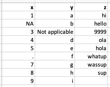
Spécification des NAs

read_csv("data/df-na.csv", 
         na = c("", "NA", ".", "9999", "Not applicable"))

# A tibble: 9 × 3
      x y     z     
  <dbl> <chr> <chr> 
1     1 a     hi    
2    NA b     hello 
3     3 <NA>  <NA>  
4     4 d     ola   
5     5 e     hola  
6    NA f     whatup
7     7 g     wassup
8     8 h     sup   
9     9 i     <NA>

Spécification des types de chaque colonne

read_csv("data/df-na.csv", col_types = list(col_double(), 
                                            col_character(), 
                                            col_character()))

# A tibble: 9 × 3
      x y              z     
  <dbl> <chr>          <chr> 
1     1 a              hi    
2    NA b              hello 
3     3 Not applicable 9999  
4     4 d              ola   
5     5 e              hola  
6    NA f              whatup
7     7 g              wassup
8     8 h              sup   
9     9 i              <NA>

Les types de colonnes

Fonction	Types de données
`col_character()`	Chaine de caractères
`col_date()`	Date
`col_datetime()`	POSIXct (date-time)
`col_double()`	Double (numeric)
`col_factor()`	Factor
`col_guess()`	Laisse readr deviner ( par défaut)
`col_integer()`	Entier
`col_logical()`	Logique
`col_number()`	Nombre et texte mélangés
`col_numeric()`	Double ou entier
`col_skip()`	Ne pas lire la colonne
`col_time()`	Temps

Jointure de données

Kesako

Lorsque nous avons des données dans plusieurs fichiers/tables, il est souvent nécessaire de les combiner.

Données: Les femmes dans la science

Nous avons des informations sur 10 femmes qui ont changé le monde. Les informations sont réparties dans trois fichiers:

professions.csv: Information sur la profession de chacune
dates.csv: date de naissance et de décès de chacune
works.csv: Ce qu’elles ont fait pour changer le monde

`professions.csv`

professions <- read_csv("data/scientists/professions.csv")
professions

# A tibble: 10 × 2
   name               profession                        
   <chr>              <chr>                             
 1 Ada Lovelace       Mathematician                     
 2 Marie Curie        Physicist and Chemist             
 3 Janaki Ammal       Botanist                          
 4 Chien-Shiung Wu    Physicist                         
 5 Katherine Johnson  Mathematician                     
 6 Rosalind Franklin  Chemist                           
 7 Vera Rubin         Astronomer                        
 8 Gladys West        Mathematician                     
 9 Flossie Wong-Staal Virologist and Molecular Biologist
10 Jennifer Doudna    Biochemist

`dates.csv`

dates <- read_csv("data/scientists/dates.csv")
dates

# A tibble: 8 × 3
  name               birth_year death_year
  <chr>                   <dbl>      <dbl>
1 Janaki Ammal             1897       1984
2 Chien-Shiung Wu          1912       1997
3 Katherine Johnson        1918       2020
4 Rosalind Franklin        1920       1958
5 Vera Rubin               1928       2016
6 Gladys West              1930         NA
7 Flossie Wong-Staal       1947         NA
8 Jennifer Doudna          1964         NA

`works.csv`

works <- read_csv("data/scientists/works.csv")
works

# A tibble: 9 × 2
  name               known_for                                                  
  <chr>              <chr>                                                      
1 Ada Lovelace       first computer algorithm                                   
2 Marie Curie        theory of radioactivity,  discovery of elements polonium a…
3 Janaki Ammal       hybrid species, biodiversity protection                    
4 Chien-Shiung Wu    confim and refine theory of radioactive beta decy, Wu expe…
5 Katherine Johnson  calculations of orbital mechanics critical to sending the …
6 Vera Rubin         existence of dark matter                                   
7 Gladys West        mathematical modeling of the shape of the Earth which serv…
8 Flossie Wong-Staal first scientist to clone HIV and create a map of its genes…
9 Jennifer Doudna    one of the primary developers of CRISPR, a ground-breaking…

Ce que nous voulons comme output

# A tibble: 10 × 5
   name               profession                 birth_year death_year known_for
   <chr>              <chr>                           <dbl>      <dbl> <chr>    
 1 Ada Lovelace       Mathematician                      NA         NA first co…
 2 Marie Curie        Physicist and Chemist              NA         NA theory o…
 3 Janaki Ammal       Botanist                         1897       1984 hybrid s…
 4 Chien-Shiung Wu    Physicist                        1912       1997 confim a…
 5 Katherine Johnson  Mathematician                    1918       2020 calculat…
 6 Rosalind Franklin  Chemist                          1920       1958 <NA>     
 7 Vera Rubin         Astronomer                       1928       2016 existenc…
 8 Gladys West        Mathematician                    1930         NA mathemat…
 9 Flossie Wong-Staal Virologist and Molecular …       1947         NA first sc…
10 Jennifer Doudna    Biochemist                       1964         NA one of t…

Types de jointures

left_join(): Retourne toutes les lignes de la première table et les lignes correspondantes de la deuxième table
right_join(): Retourne toutes les lignes de la deuxième table et les lignes correspondantes de la première table
inner_join(): Retourne les lignes qui ont une correspondance dans les deux tables
full_join(): Retourne toutes les lignes des deux tables
semi_join(): Retourne toutes les lignes de la première table qui ont une correspondance dans la deuxième table
anti_join(): Retourne toutes les lignes de la première table qui n’ont pas de correspondance dans la deuxième table

Pour l’exemple…

# A tibble: 3 × 2
     id value_x
  <dbl> <chr>  
1     1 x1     
2     2 x2     
3     3 x3

# A tibble: 3 × 2
     id value_y
  <dbl> <chr>  
1     1 y1     
2     2 y2     
3     4 y4

`left_join()`

left_join(x, y)

# A tibble: 3 × 3
     id value_x value_y
  <dbl> <chr>   <chr>  
1     1 x1      y1     
2     2 x2      y2     
3     3 x3      <NA>

`left_join()`

professions %>%
  left_join(dates)

# A tibble: 10 × 4
   name               profession                         birth_year death_year
   <chr>              <chr>                                   <dbl>      <dbl>
 1 Ada Lovelace       Mathematician                              NA         NA
 2 Marie Curie        Physicist and Chemist                      NA         NA
 3 Janaki Ammal       Botanist                                 1897       1984
 4 Chien-Shiung Wu    Physicist                                1912       1997
 5 Katherine Johnson  Mathematician                            1918       2020
 6 Rosalind Franklin  Chemist                                  1920       1958
 7 Vera Rubin         Astronomer                               1928       2016
 8 Gladys West        Mathematician                            1930         NA
 9 Flossie Wong-Staal Virologist and Molecular Biologist       1947         NA
10 Jennifer Doudna    Biochemist                               1964         NA

`right_join()`

right_join(x, y)

# A tibble: 3 × 3
     id value_x value_y
  <dbl> <chr>   <chr>  
1     1 x1      y1     
2     2 x2      y2     
3     4 <NA>    y4

`right_join()`

professions %>%
  right_join(dates)

# A tibble: 8 × 4
  name               profession                         birth_year death_year
  <chr>              <chr>                                   <dbl>      <dbl>
1 Janaki Ammal       Botanist                                 1897       1984
2 Chien-Shiung Wu    Physicist                                1912       1997
3 Katherine Johnson  Mathematician                            1918       2020
4 Rosalind Franklin  Chemist                                  1920       1958
5 Vera Rubin         Astronomer                               1928       2016
6 Gladys West        Mathematician                            1930         NA
7 Flossie Wong-Staal Virologist and Molecular Biologist       1947         NA
8 Jennifer Doudna    Biochemist                               1964         NA

`full_join()`

full_join(x, y)

# A tibble: 4 × 3
     id value_x value_y
  <dbl> <chr>   <chr>  
1     1 x1      y1     
2     2 x2      y2     
3     3 x3      <NA>   
4     4 <NA>    y4

`full_join()`

professions %>%
  full_join(works)

# A tibble: 10 × 3
   name               profession                         known_for              
   <chr>              <chr>                              <chr>                  
 1 Ada Lovelace       Mathematician                      first computer algorit…
 2 Marie Curie        Physicist and Chemist              theory of radioactivit…
 3 Janaki Ammal       Botanist                           hybrid species, biodiv…
 4 Chien-Shiung Wu    Physicist                          confim and refine theo…
 5 Katherine Johnson  Mathematician                      calculations of orbita…
 6 Rosalind Franklin  Chemist                            <NA>                   
 7 Vera Rubin         Astronomer                         existence of dark matt…
 8 Gladys West        Mathematician                      mathematical modeling …
 9 Flossie Wong-Staal Virologist and Molecular Biologist first scientist to clo…
10 Jennifer Doudna    Biochemist                         one of the primary dev…

`inner_join()`

inner_join(x, y)

# A tibble: 2 × 3
     id value_x value_y
  <dbl> <chr>   <chr>  
1     1 x1      y1     
2     2 x2      y2

`inner_join()`

professions %>%
  inner_join(dates)

# A tibble: 8 × 4
  name               profession                         birth_year death_year
  <chr>              <chr>                                   <dbl>      <dbl>
1 Janaki Ammal       Botanist                                 1897       1984
2 Chien-Shiung Wu    Physicist                                1912       1997
3 Katherine Johnson  Mathematician                            1918       2020
4 Rosalind Franklin  Chemist                                  1920       1958
5 Vera Rubin         Astronomer                               1928       2016
6 Gladys West        Mathematician                            1930         NA
7 Flossie Wong-Staal Virologist and Molecular Biologist       1947         NA
8 Jennifer Doudna    Biochemist                               1964         NA

Si on reprend…

professions %>%
  left_join(dates) %>%
  left_join(works)

# A tibble: 10 × 5
   name               profession                 birth_year death_year known_for
   <chr>              <chr>                           <dbl>      <dbl> <chr>    
 1 Ada Lovelace       Mathematician                      NA         NA first co…
 2 Marie Curie        Physicist and Chemist              NA         NA theory o…
 3 Janaki Ammal       Botanist                         1897       1984 hybrid s…
 4 Chien-Shiung Wu    Physicist                        1912       1997 confim a…
 5 Katherine Johnson  Mathematician                    1918       2020 calculat…
 6 Rosalind Franklin  Chemist                          1920       1958 <NA>     
 7 Vera Rubin         Astronomer                       1928       2016 existenc…
 8 Gladys West        Mathematician                    1930         NA mathemat…
 9 Flossie Wong-Staal Virologist and Molecular …       1947         NA first sc…
10 Jennifer Doudna    Biochemist                       1964         NA one of t…

Tidy data

Happy families are all alike; every unhappy family is unhappy in its own way. – Leo Tolstoy

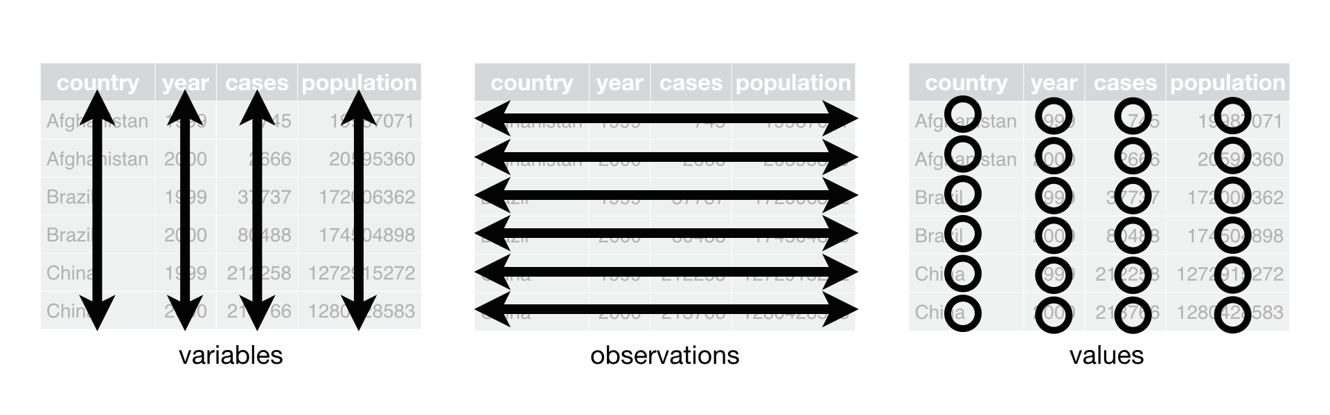
Qu’est ce que des données Tidy ?

Chaque variable est une colonne
Chaque observation est une ligne
Chaque valeur est une cellule

Tidy data

(Wickham et al., 2023, chap. 5)

Exemples

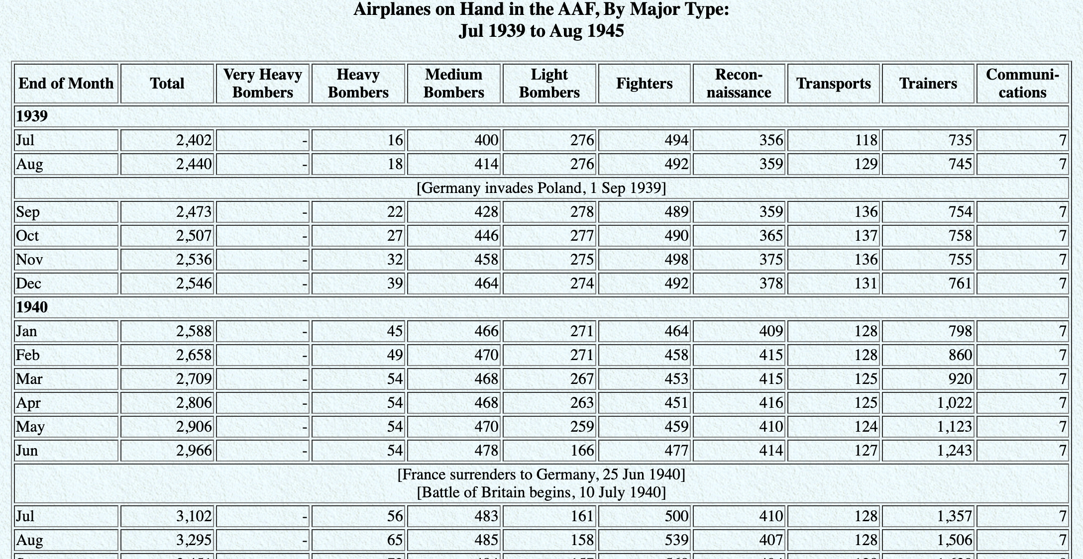
En quoi ces données ne sont pas tidy ?

Source: Army Air Forces Statistical Digest, WWII

En quoi ces données ne sont pas tidy ?

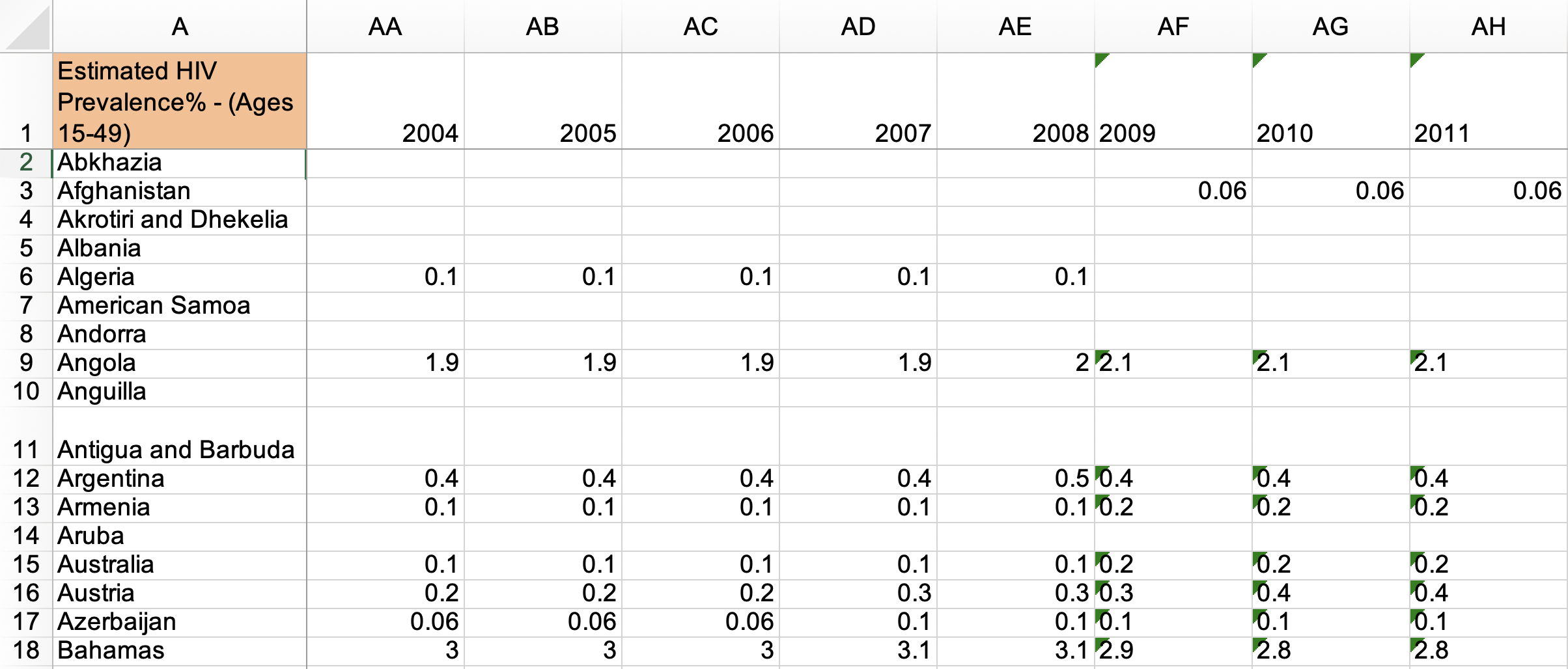
Source: Gapminder, Estimated HIV prevalence among 15-49 year olds

En quoi ces données ne sont pas tidy ?

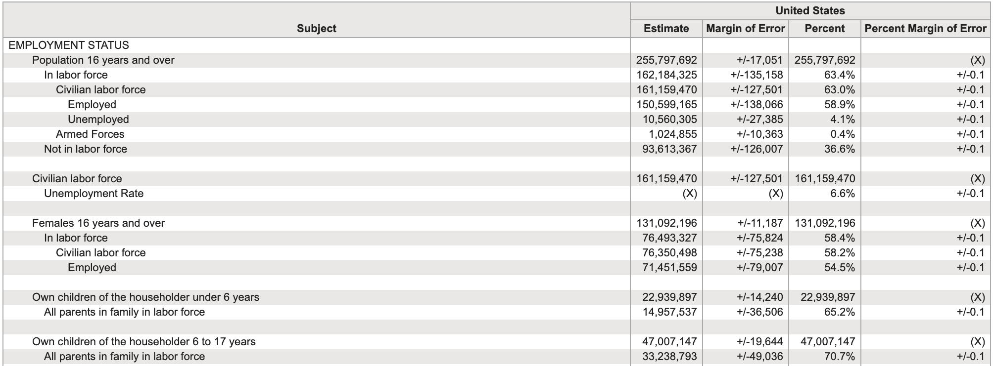
Source: US Census Fact Finder, General Economic Characteristics, ACS 2017

Tidying data

Ce qu’on a…

# A tibble: 2 × 4
  customer_id item_1 item_2       item_3
        <dbl> <chr>  <chr>        <chr> 
1           1 bread  milk         banana
2           2 milk   toilet paper <NA>

Ce qu’on veut…

# A tibble: 6 × 3
  customer_id item_no item        
        <dbl> <chr>   <chr>       
1           1 item_1  bread       
2           1 item_2  milk        
3           1 item_3  banana      
4           2 item_1  milk        
5           2 item_2  toilet paper
6           2 item_3  <NA>

Pour Tidyer: Tidyr

Tidyr permet de transformer les données pour les Tidy :

Faire pivoter les données
Séparer ou combiner des colonnes
Imbriquer/Désimbriquer des colonnes
Préciser commenter traiter les NA

Pivoter les données

Wide vs Long

Forme large :

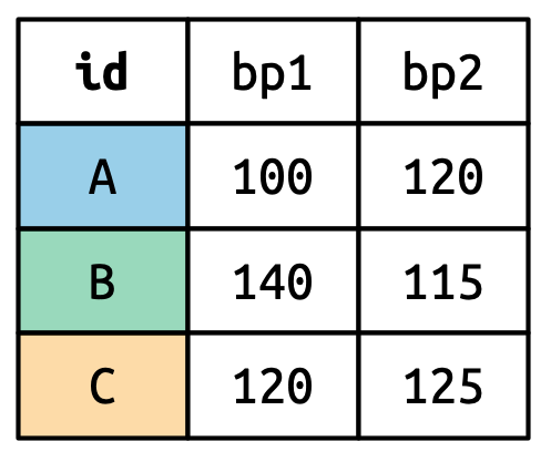
Forme longue :

Source: (Wickham et al., 2023, chap. 5)

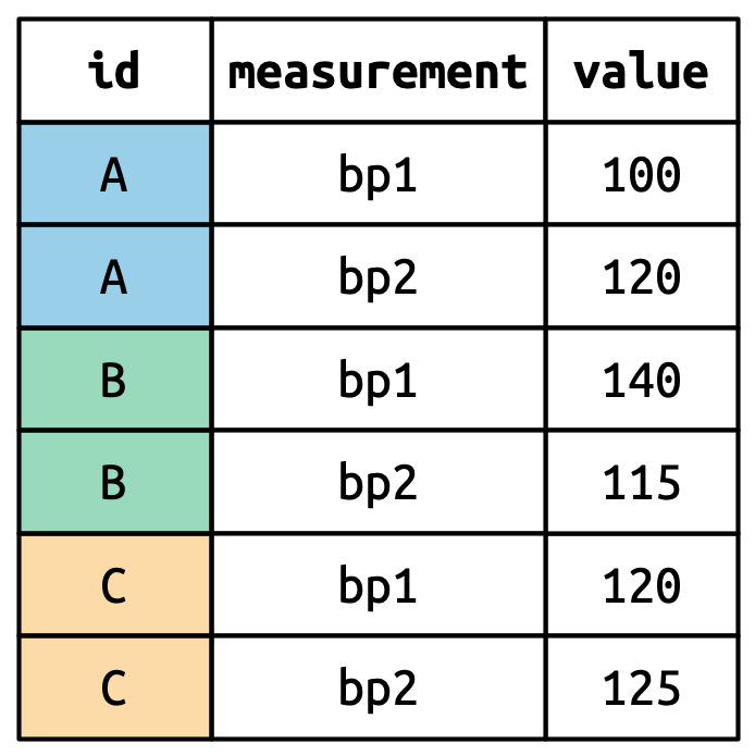
Wide vs Long

Wide

Plus de colonnes

# A tibble: 2 × 4
  customer_id item_1 item_2       item_3
        <dbl> <chr>  <chr>        <chr> 
1           1 bread  milk         banana
2           2 milk   toilet paper <NA>

Long

Plus de lignes

# A tibble: 6 × 3
  customer_id item_no item        
        <dbl> <chr>   <chr>       
1           1 item_1  bread       
2           1 item_2  milk        
3           1 item_3  banana      
4           2 item_1  milk        
5           2 item_2  toilet paper
6           2 item_3  <NA>

`pivot_longer()`

data : Comme d’habitude
cols : Colonne à pivoter
names_to : Nom de la colonne où les variables vont être envoyées
values_to : Nom de la colonne où les valeurs vont être envoyées

pivot_longer(
  data, 
  cols, 
  names_to = "name", 
  values_to = "value"
  )

Customer \(\rightarrow\) purchases

purchases <- customers %>%
  pivot_longer(
    cols = item_1:item_3,  # variables item_1 à item_3
    names_to = "item_no",  # Noms des colonnes -> dans une nouvelle colonne item_no
    values_to = "item"     # valeurs pour chaque colonne -> dans une nouvelle colonne item
    )

purchases

# A tibble: 6 × 3
  customer_id item_no item        
        <dbl> <chr>   <chr>       
1           1 item_1  bread       
2           1 item_2  milk        
3           1 item_3  banana      
4           2 item_1  milk        
5           2 item_2  toilet paper
6           2 item_3  <NA>

`pivot_wider()`

data : Comme d’habitude
names_from : Colonne contenant les noms de colonnes
values_from : Colonne contenant les valeurs

purchases %>%
  pivot_wider(
    names_from = item_no,
    values_from = item
  )

# A tibble: 2 × 4
  customer_id item_1 item_2       item_3
        <dbl> <chr>  <chr>        <chr> 
1           1 bread  milk         banana
2           2 milk   toilet paper <NA>

Références

Wickham, H., Çetinkaya-Rundel, M. and Grolemund, G. (2023). R for Data Science (2nd ed.). O’Reilly Media, Inc. https://r4ds.hadley.nz/